
Coding tokens
The linguistic subfield of language variation and change studies linguistic variables: speakers’ choices between multiple linguistic forms that exist in the same linguistic environment. For example, some speakers of Pittsburgh English pronounce the /aw/ vowel (the vowel sound in words like out and downtown) more like “ah” (stereotyped as “aht” and “dahntahn”). The multiple forms of the /aw/ variable (“aw” and “ah”) are known as variants. In order to research this variable, a researcher has to listen to every token of /aw/ and manually identify whether the speaker pronounced it as “aw” or “ah”. This process, which is called coding, is often tedious and time-consuming.
Fortunately, APLS makes coding much easier and faster. On this page, we’ll discuss three common coding scenarios:
- Variables for which codes can be extracted from annotations without you needing to manually code tokens
- In some cases, you may need to categorize or relabel annotations
- Variables that can be coded based on the text of the transcript alone
-
Variables for which you need to listen to transcript audio in order to code them
This is often the most challenging of the three coding scenarios. To make it easier and faster, we’ve created a program,
CodeTokens.praat.
While this page focuses mosly on coding variants, these scenarios can also apply to predictors. Not covered on this page is measuring tokens’ acoustic properties, which you might want to do instead of (or in addition to) coding them.
If you haven’t yet, read the documentation section on searching the corpus and the page on exporting data before reading this page.
On this page
The coding workflow
The coding (and data analysis) workflow usually looks something like this:
- Create a search where each match is one token of the variable you’re interested in, for the participants and/or transcripts in your sample.
- This can take some trial and error!
- Export search results to CSV.
- If coding by listening to audio, export utterances as Praat TextGrids and audio files as well.
- If needed, enter codes in a new CSV column.
- CSVs can be read and edited in spreadsheet programs like Microsoft Excel, Numbers for Mac, or Google Sheets.
- If coding by listening to audio, you can use the
CodeTokens.praatPraat script to make this much faster.
-
If needed, code predictors (aka independent variables or constraints) in new CSV columns.
At this point, you should have a CSV file that has:
- One row per token of the variable you’re interested in
- One column with variant codes
- One column per predictor you want to use in your analysis
- Any other columns you want
This will enable you to:
- Use a program like Excel or R for statistical modeling and/or data visualization.
Coding tokens by extracting annotations
In this scenario, annotations that are already in APLS provide the codes. This works well for many lexical variables (like slippy vs. slippery), morphological variables (like don’t vs. doesn’t), and syntactic variables (like will vs. going to vs. gonna). In each of those cases, you can export annotations that are on the orthography layer.
If you want to use orthography annotations for your codes, consult the APLS transcription convention to understand which distinctions the orthography layer does or doesn’t make. For example, transcribers were permitted to use some colloquial spellings, such as gonna; as a result, you can extract will vs. going to vs. gonna codes from orthography annotations. However, transcribers were not permitted to use “eye dialect” spellings like warsh or jumpin’, so you can’t get those distinctions from orthography annotations.
In some cases, you still might need to categorize or relabel exported annotations into variants in order to get your codes. For example, if you’re looking at a set of “Pittsburghese” lexical items, you might need to create a new CSV column that categorizes some orthography annotations as Pittsburgh (such as slippy, nebby, sweeper) and others as non-Pittsburgh (such as slippery, nosey, vacuum). This is easier to do if you use a formula in a spreadsheet program like Excel or a programming language like R, as discussed below.
With these variables, the tricky thing isn’t coding, it’s figuring out which forms are actual tokens of the variable vs. unrelated forms. This description of which forms count as tokens of the variable is known as the variable context or envelope of variation. In some cases, you can encode the variable context in your search pattern. For example, if you’re investigating English future-tense variation (will vs. going to vs. gonna), you’ll want to exclude forms that aren’t in the future tense (like “a strong will” or “going to the store”). In this particular example, you can use the part_of_speech layer to only include will tokens that are modal verbs (part_of_speech MD) and going to tokens where the to is an infinitival marker (part_of_speech TO).
In other situations, you might have to consult the context of the words in the transcript to manually include or exclude matches. For example, let’s say you’re investigating variation in how speakers mark 3rd-person singular present-tense verbs (such as he wants vs. he want). For this variable, tokens of want with non-3rd-person-singular subjects (like you want) are outside of the variable context, because these don’t vary with wants (that is, speakers who say he want don’t also say you wants). Because APLS doesn’t currently have a layer that encodes the subject of a verb, you’ll need to read the transcript to see which tokens of want actually have a 3rd-person singular subject.
Not for phonological variables
This scenario generally doesn’t apply to phonological variables (like [ɪŋ] vs. [ɪn] endings in words like working or something). Instead, these variables need to be coded by listening to audio.
This is because annotations on phonological layers like segment are phonemic, not phonetic. To generate the segment layer, APLS first uses pronouncing dictionaries to match each word’s orthography annotation to a phonemic representation (like /ˈwɝɹkɪŋ/ for working, /ˈsʌmθɪŋ/ for something), then uses the HTK algorithm to find the start and end time of each of these sounds. While some orthography annotations have multiple phonemic representations in the dictionary, this is restricted to homophones (like desert as /dəˈzɝt/ vs. /ˈdɛzɚt/) or reduced vs. unreduced pronounciations of highly common words (like to as /tə/ vs. /ˈtu/). As a result, working and something are always represented in APLS as ending with /ɪŋ/, regardless of whether the speaker said [wɝɹkɪŋ] or [wɝɹkɪn].
User-contributed codes
APLS currently contains 1 layer that consists of user-contributed annotations: coronal_stop_deletion. This layer can be found in the user_contrib project. However, don’t just take these codes at face value; they may represent different decisions than you (or other researchers) would have made about which tokens to include in the variable context, how many variants there are, coding criteria, and even the codes of individual tokens. If you want to use a user-contributed layer, carefully read its description in the layer field guide (linked above), and consider recoding a randomly selected subset of codes to check your agreement with the original coder(s).
Coding tokens by reading context
In this scenario, coding is done manually by looking at the context of the words in the transcript. In the previous scenario, the codes come from the form of the token (that is, the annotation); in this scenario, the codes come from the meaning or function of the token. This works well for variables such as like, which can be a verb on its own (“I would like that”), part of the quotative verb be like (“she was like, ‘what do you mean?’”), a preposition (“things like that”), a subordinating conjunction (“like I said”), or a discourse particle (“my like role model”).
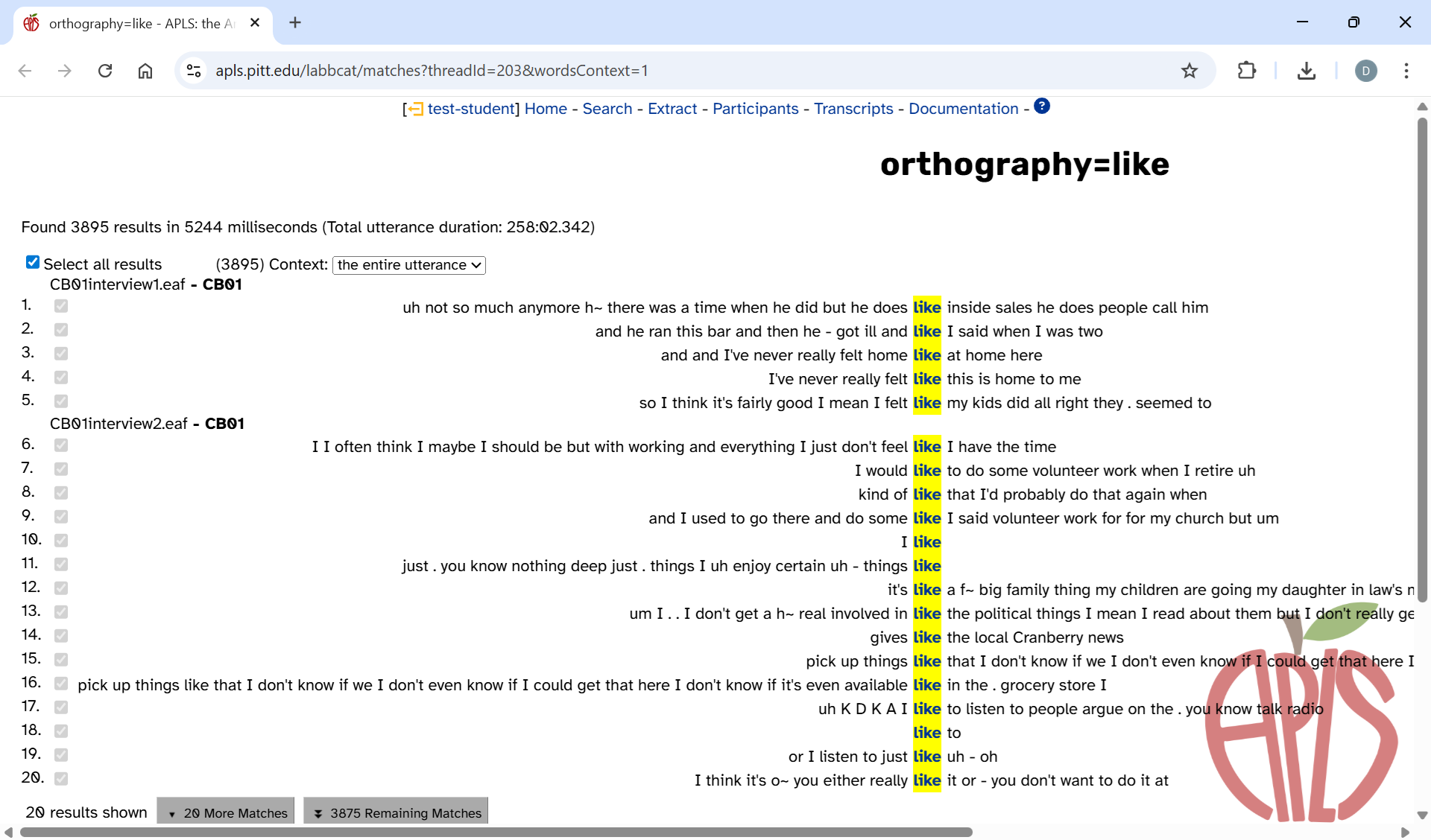
On the Search results page, you can use the context selector to view the entire text of the utterance that contains each token. Here’s what that looks like for a simple search for like on the orthography layer (with the Only include matches from the main participant in a transcript match option selected):
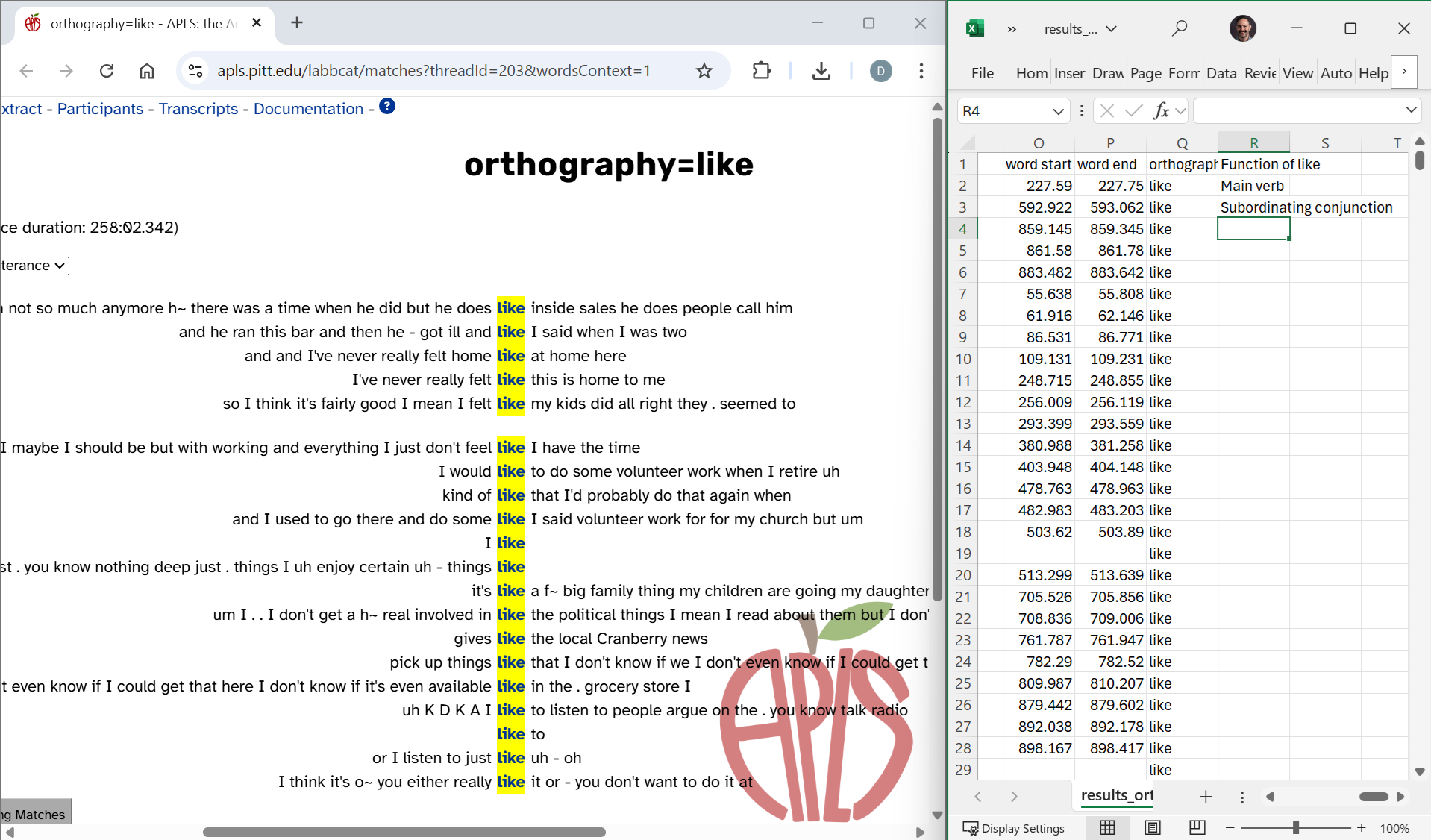
Then you can enter codes in a new column in your results CSV file. If you’re using Windows, you can use Snap to put your browser and CSV file side-by-side:
You might also find it convenient to hide columns in the CSV file (Excel instructions) so you can make sure you’re coding the correct row:
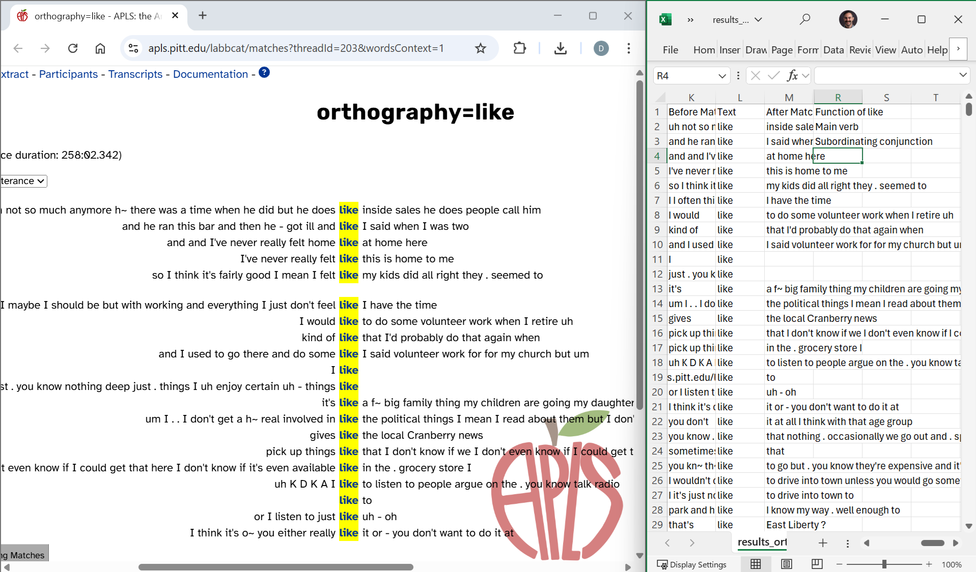
Don’t delete columns—you might want them later! Hide them instead.
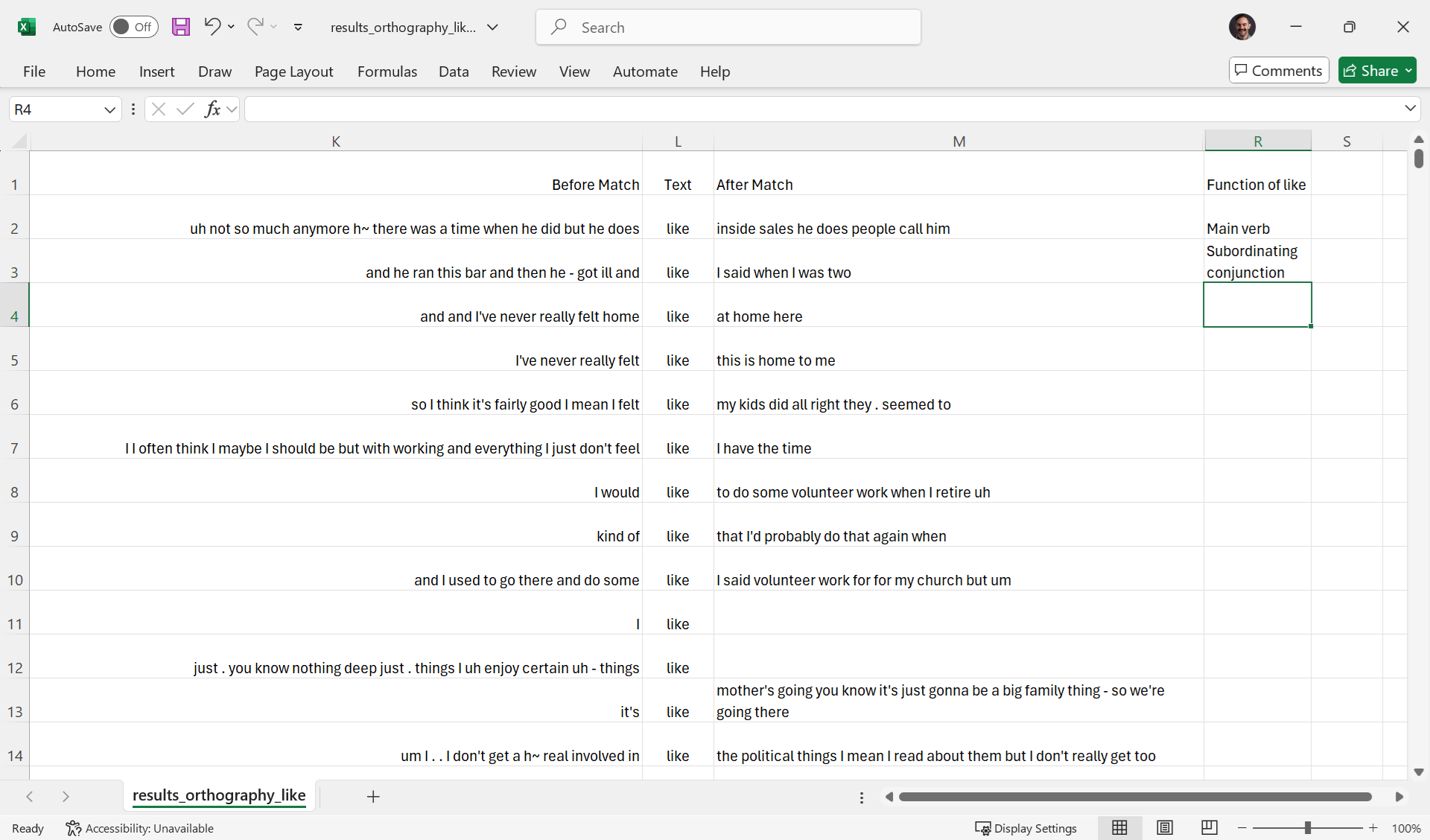
Since the Before Match, Text, and After Match columns show the same search context that’s on the Search results page, you can use only the CSV file if you don’t want to use multiple windows. This can be useful if you have a lot of tokens to code and can’t count on internet access the whole time. That said, it does take some tweaking of the display settings to look nice. Here’s what it looks like in Excel when you hide all columns except those three and the coding column, adjust the column widths, select Wrap text so the whole context is visible when it’s long, and adjust row heights so they’re not too tall:
If you want to return to the Search results page interface after you’ve closed APLS, you can reupload your CSV file to the Extract data based on search results page (https://apls.pitt.edu/labbcat/matches/upload).
Viewing tokens on the Transcript page
In some cases, you may need more context than is available on the Search results page or in the Before Match/After Match CSV columns. For example, the third like search result is ambiguous without knowing what comes after “like at home here”. Clicking on a match link on the Search results page will open the Transcript page in a new tab and highlight/scroll to that token. Here’s what it looks like when you click the third like match link:
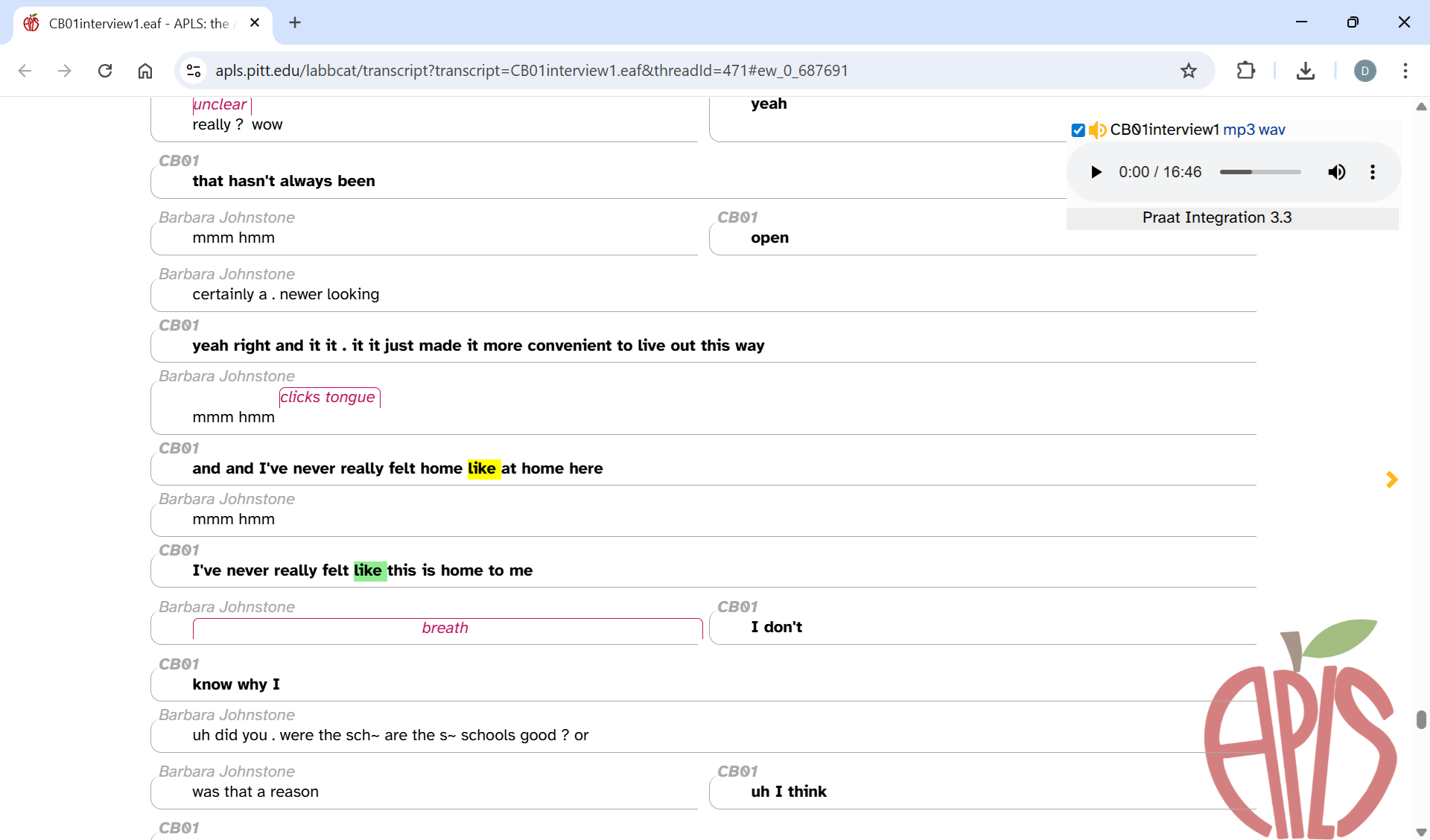
As you can see, the like in “like at home here” has been highlighted in yellow. The next like token (in “like this is home”) has been highlighted in green, and if you scroll elsewhere in the transcript, you’ll see other like tokens highlighted in green too. If you’re working with a CSV, you can access these links in the URL column.
Like on the Search results page, the CSV
URLlinks open the Transcript page, scroll to that token, and highlight it in yellow. However, other tokens aren’t highlighted in green. This is because of the same reason that the Search results page can’t be permalinked. Highlighting other tokens requires APLS to save stored data on search tasks, and once a user closes the Search or Search results page, APLS cleans out the stored search task data to save server space.
Occasionally, even reading tokens on the Transcript page may not be enough to tell the difference between two functions of like, and you need to hear the speaker’s intonation and speech rhythm to code a token. In that case, you can listen to the token in context by playing the utterance audio from the word menu.
Coding tokens by listening to audio
In this scenario, coding is done manually by listening to how speakers produce tokens of a variable. This is known as auditory coding. Auditory coding works well for phonological variables (like [ɪŋ] vs. [ɪn] endings in words like working or something) and suprasegmental variables (like creaky voice vs. modal voice). In other words, auditory coding is necessary for coding variables where the different variants don’t correspond to annotations in APLS and can’t be determined from reading the transcript. (See above for why phonological annotations are phonemic, not phonetic.)
One way to do auditory coding in APLS would be to open each search result on the Transcript page and use the word menu to play just the utterance that contains the token. But we’ve created a faster way: CodeTokens.praat. CodeTokens.praat is a program (running within Praat) that makes coding faster and easier by seamlessly integrating with the APLS Search results page, playing tokens one-at-a-time, providing a graphical user interface for selecting variants, and writing your codes to a CSV file:
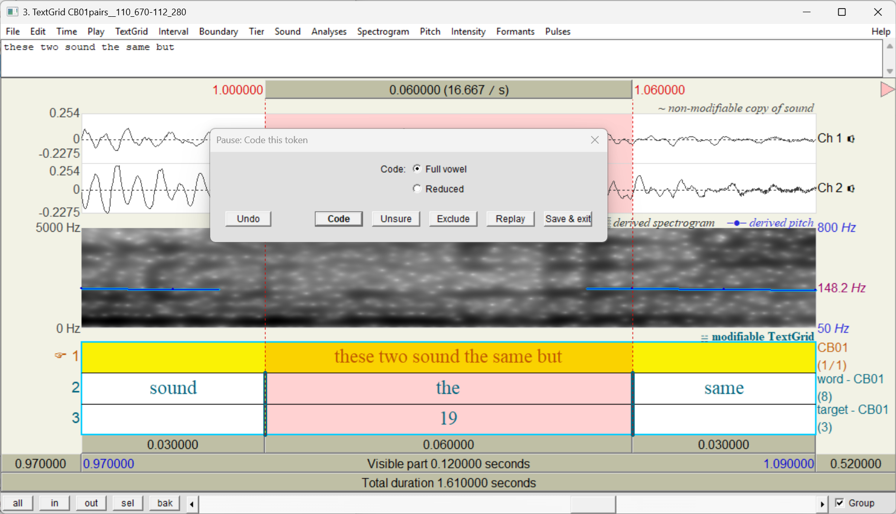
To learn more, visit the CodeTokens.praat documentation page.
Coding predictors
The same token-coding scenarios discussed above apply to coding predictors (aka independent variables or constraints):
- Coding predictors by extracting annotations. Works well when the predictor can come:
- Directly from annotations on an APLS layer (like frequency_in_corpus) or attribute (like gender)
- From relabeled annotations (like providing nicer labels for stress markers or part_of_speech tags)
- From categorized annotations (like categorizing morphemes annotations into
past tensevs.non-past tense, or putting speech_rate annotations into bins likefast,medium, andslow)
Unlike coding tokens, this scenario can apply to phonological predictors, as long as the predictor is defined on the level of phonemes rather than surface representations. For example, in American English, the vowel /u/ (as in goose) is often pronounced with the tongue further forward in the mouth when the preceding sound is a coronal consonant like /t/ than a non-coronal consonant like /p/. You can get this information by categorizing prec_segment annotations into
coronalvs.non-coronal. - Coding predictors by reading context. Works well for predictors that are difficult to extract from APLS annotations, on the level of:
- Discourse (like topic or stance)
- Syntax (like the subject of a verb)
- Coding tokens by listening to context. Works well for predictors that require listening on the level of:
- Segmental phonology (like whether the vowel in the -ing ending is [ɪ] or [i])
- Suprasegmentals (like creaky voice vs. modal voice)
- Discourse (like whether a speaker is being sarcastic)
- Measuring predictors by extracting acoustic properties of each token. Works well for measurable predictors like pitch
Categorizing and relabeling annotations
As mentioned above, some variables or predictors can be coded by extracting annotations directly from APLS; while some of these can be used as-is, others need to be categorized or relabeled. Here are some examples:
- Categorizing: Labeling orthography annotations as either
Pittsburgh(such as slippy, nebby, sweeper) ornon-Pittsburgh(such as slippery, nosey, vacuum) - Categorizing: Putting speech_rate annotations into bins like
fastandslow - Relabeling: Replacing education annotations (such as
HS,BA, and> BA) with longer descriptions (such ashigh school,undergraduate, andgraduate).
All of these tasks can be accomplished more quickly and easily with a spreadsheet program like Excel or a programming language like R.
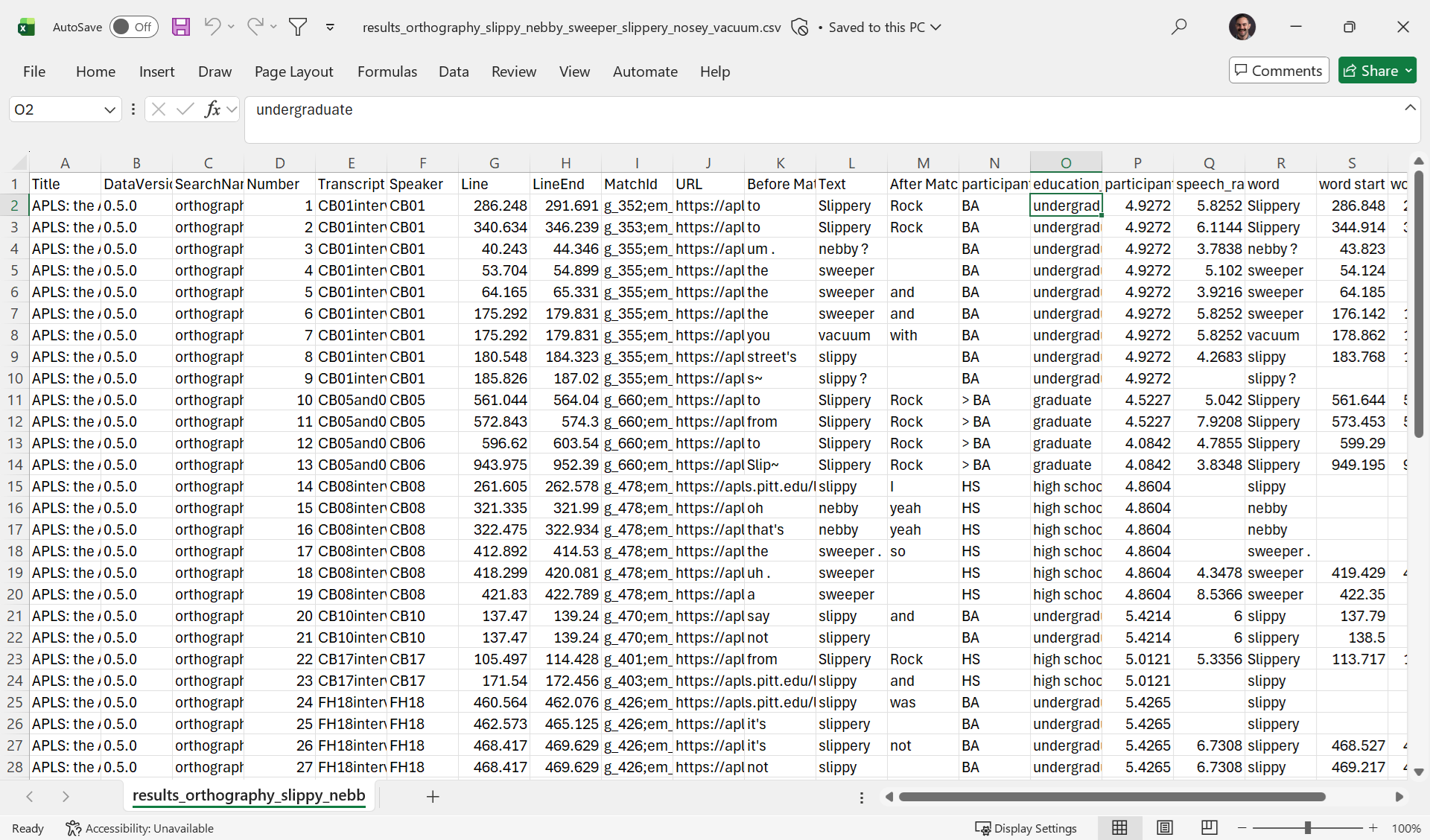
To illustrate these processes, we’ll search the orthography layer for the pattern slippy|nebby|sweeper|slippery|nosey|vacuum, with the Only include matches from the main participant in a transcript match option selected. Then we’ll export the CSV with all pre-selected metadata fields/attributes/layers, plus education, participant speech_rate, and phrase speech_rate. Here’s what that CSV looks like in Microsoft Excel:
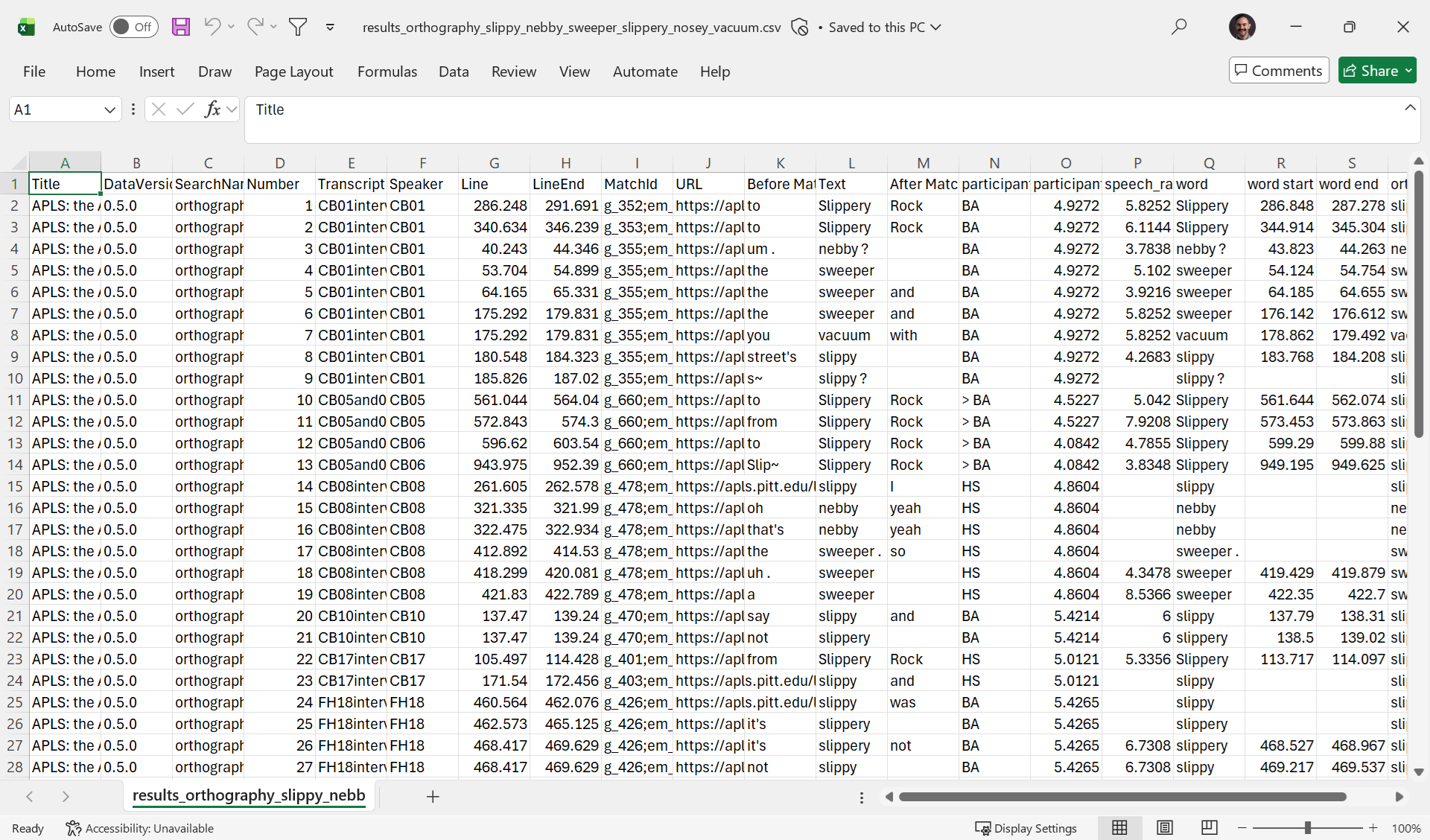
We’ll demonstrate these relabeling and categorizing steps in Microsoft Excel, but the steps are very similar in other spreadsheet programs. In particular, the Excel functions that we describe (
SWITCH,IF, andISBLANK) all exist in Google Sheets and Numbers for Mac.
Relabeling annotations
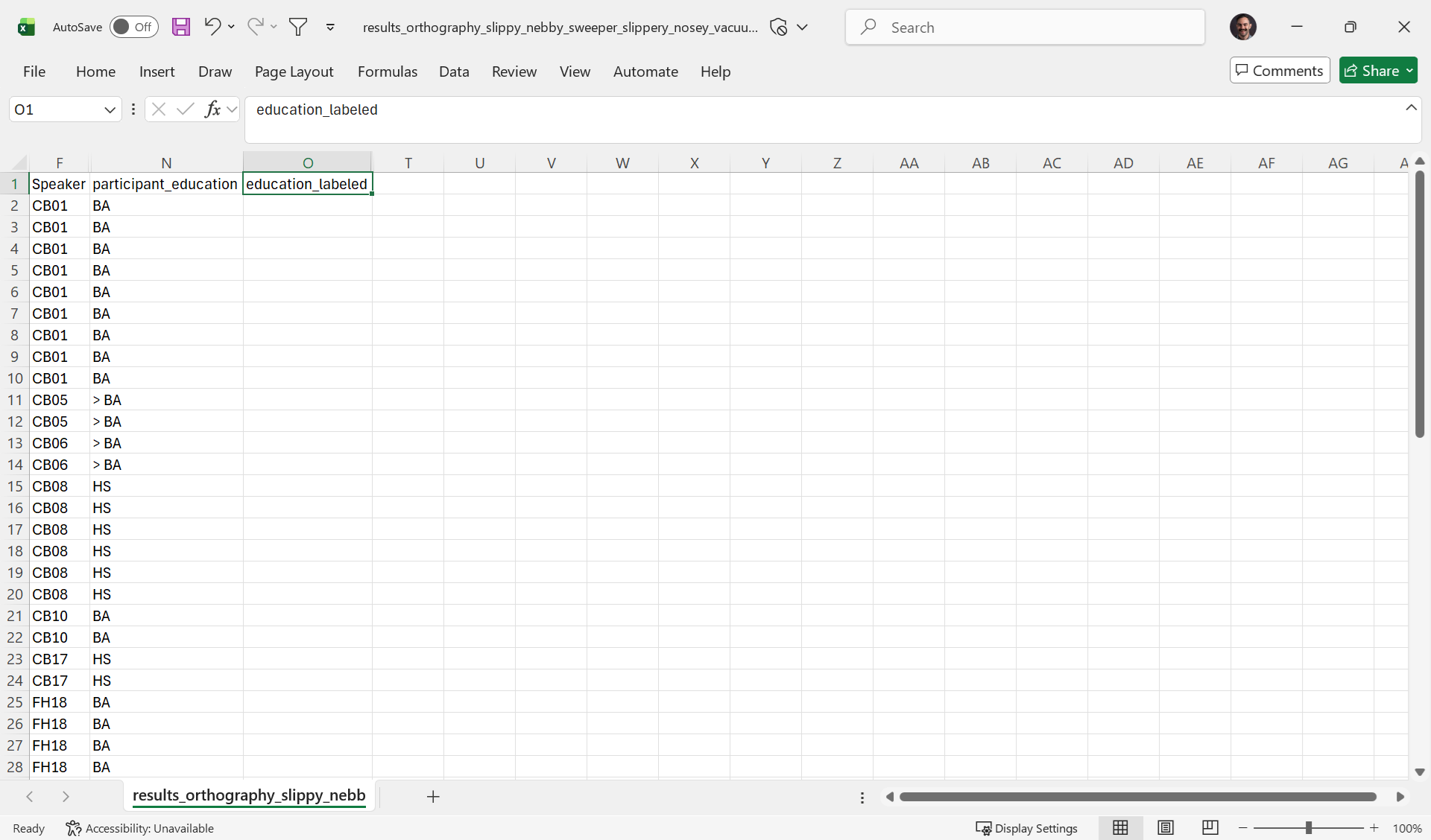
To relabel the participant_education column (column N in the above screenshot), we’ll first add a new column to its right. In Excel, you can click on the column header O, then press either Ctrl Shift + (Windows) or Cmd Shift + (Mac) to add a new blank column after participant_education. We’ll add a new column name in cell O1: education_labeled. Here’s what that looks like:
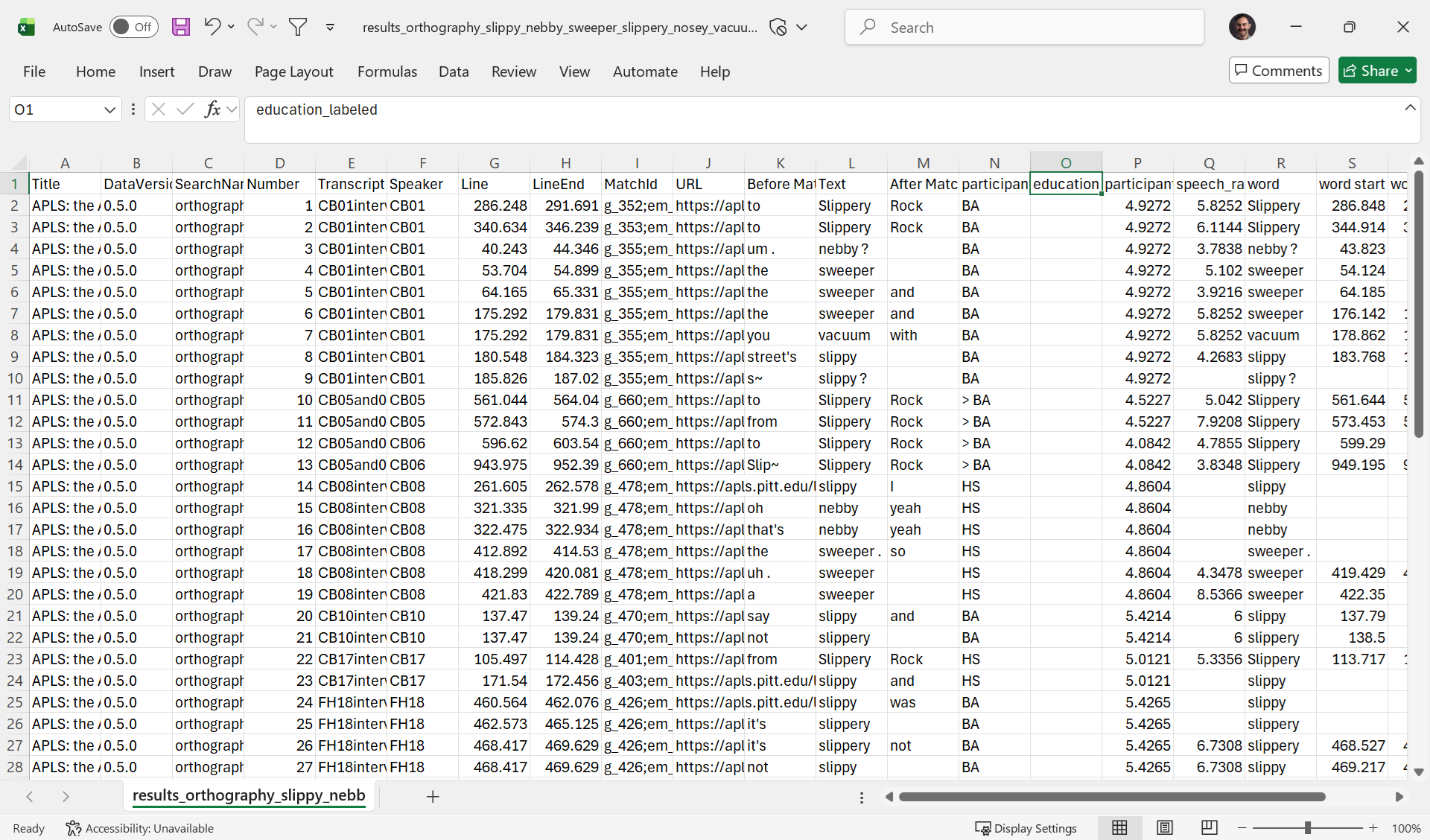
At this point, we’ll also hide columns: all but Speaker, participant_education, and education_labeled. This is just for demonstration purposes; you don’t have to do this when you relabel or categorize columns. Here’s what that looks like:
Then we can use a formula to tell Excel how to fill in the values of the new education_labeled column. In particular, we’ll tell the SWITCH function to look in the participant_education column and how to relabel the codes in that column. Here’s what it looks like if you select cell O2 and type =SWITCH(N2, "HS", "high school", "BA", "undergraduate", "> BA", "graduate", ""):
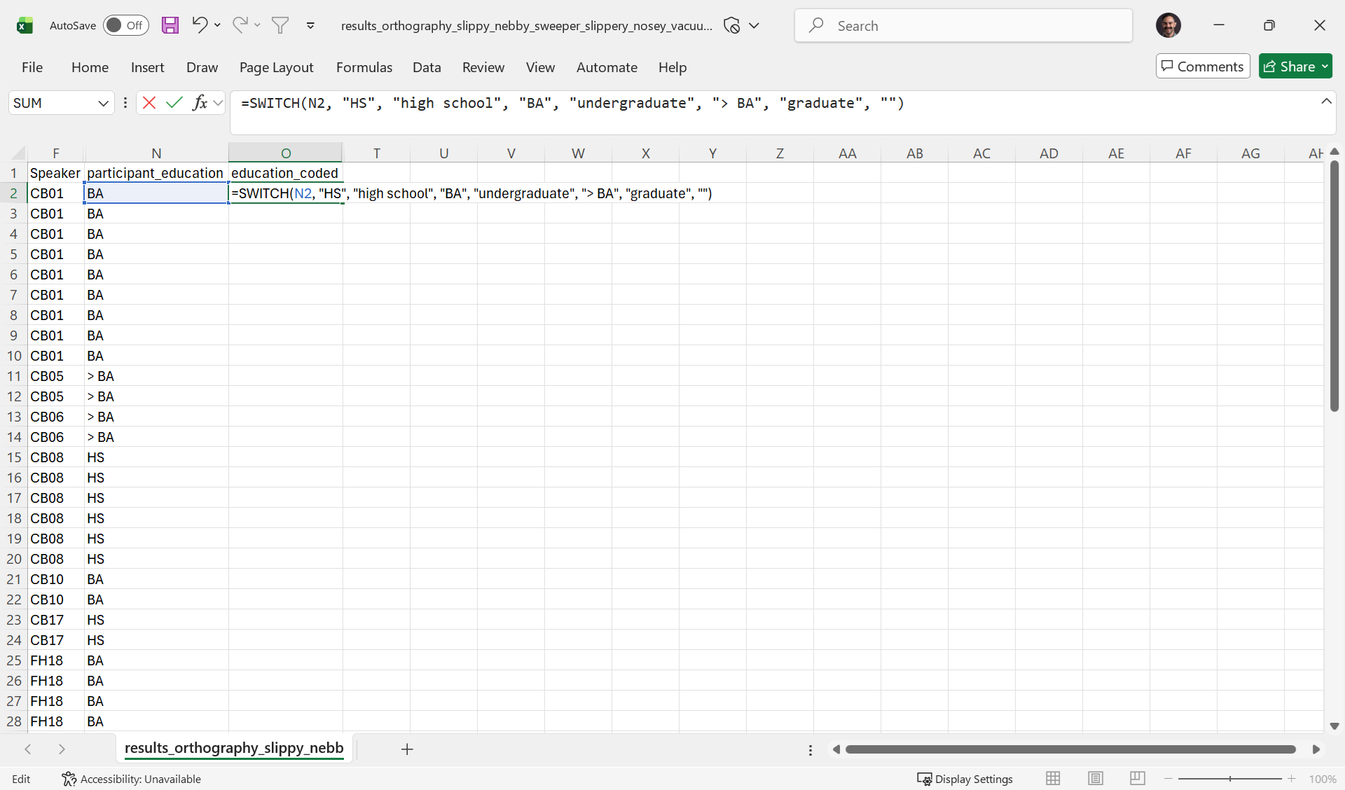
As you can see, cell N2 is highlighted in blue because it’s being referred to in the formula. If you press Enter/Return, Excel will evaluate the formula in cell O2, returning undergraduate:
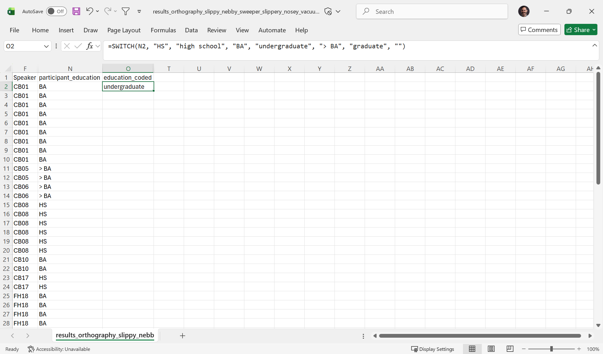
As you can see, cell O2 shows undergraduate; when O2 is highlighted, the formula bar (above the column headers) shows the =SWITCH(... formula. You can edit this formula as needed and press Enter/Return to have Excel re-evaluate it.
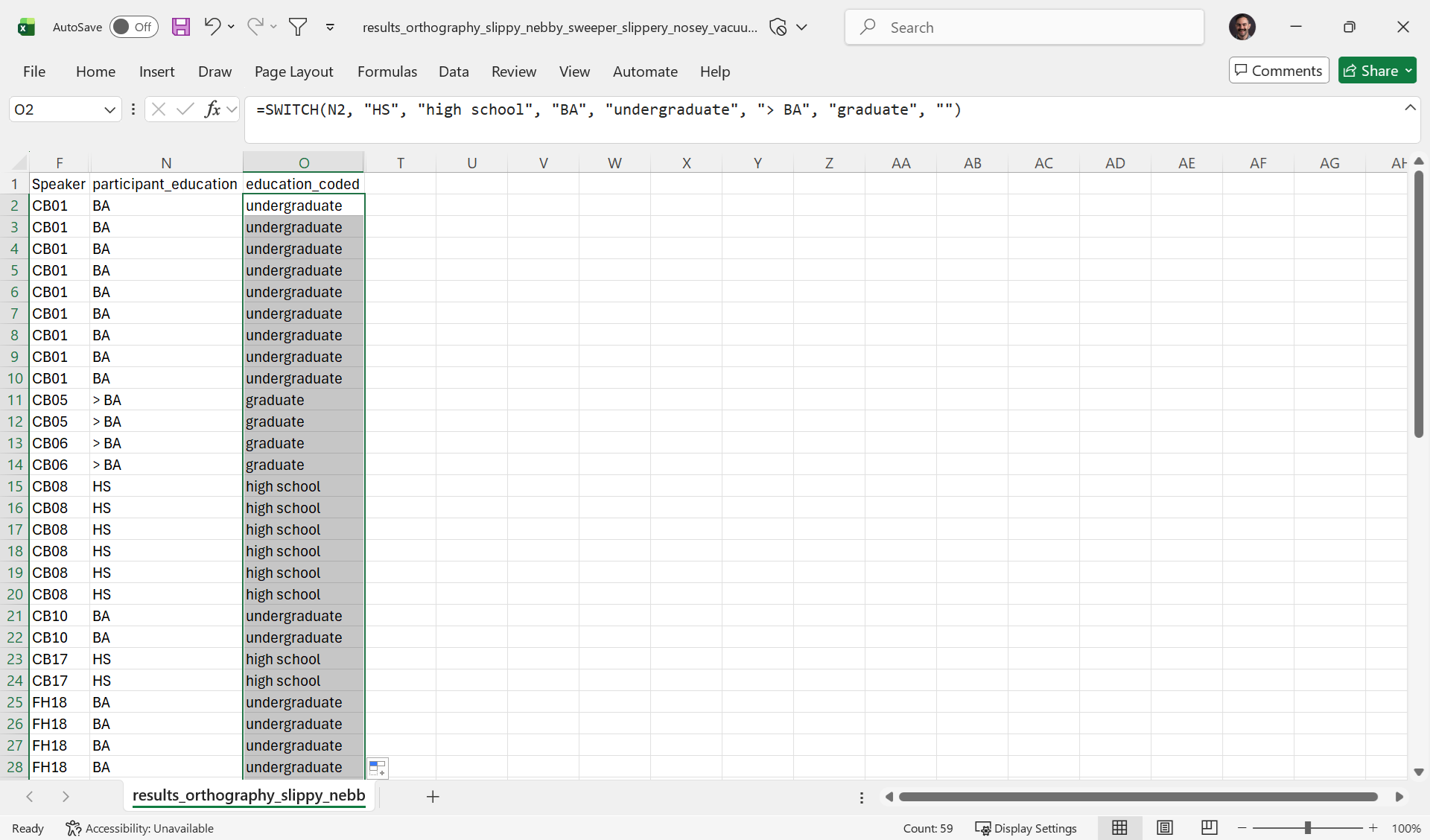
If you select O2 again and double-click the small square in the bottom-right corner (the fill handle), it will apply this formula to the rest of the cells in the column:
While you can use formulas to edit CSV files while Excel is open, only the evaluated values are saved, not the formulas. As a result, if you close Excel and reopen the CSV file, you’ll only be able to see the values. For example, cell
O2now shows justundergraduatein both the cell and the formula bar:
If you want to save the formulas as well as the values, do one of the following:
- Save the CSV file as an
.xlsxfile instead, which preserves formulas.
- If you want to re-upload the file to APLS, you’ll need to convert it back to CSV.
- Keep a “README” file on your computer, along with the other files for your project, that describes the steps needed to reproduce your data preparation and analysis.
- In our opinion, this is the better option! If you have two files, both named
results, it’s easy to lose track of which one is the “real” one. Always remember your most important collaborator.
Categorizing annotations
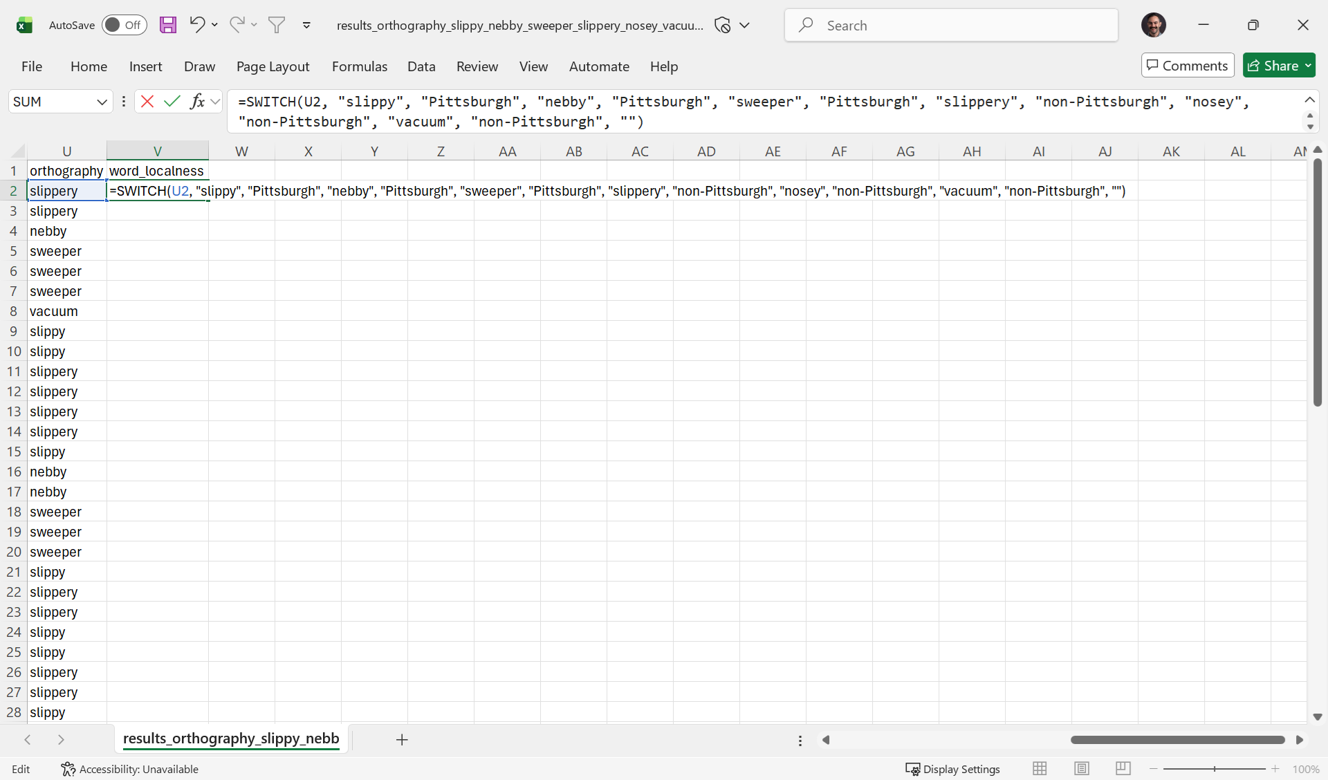
Now, let’s categorize orthography annotations as either Pittsburgh (such as slippy, nebby, sweeper) or non-Pittsburgh (such as slippery, nosey, vacuum) in a new word_localness column. Like we did with relabeling education, we can use the SWITCH function. Here’s what it looks like if you select V2 and type =SWITCH(U2, "slippy", "Pittsburgh", "nebby", "Pittsburgh", "sweeper", "Pittsburgh", "slippery", "non-Pittsburgh", "nosey", "non-Pittsburgh", "vacuum", "non-Pittsburgh", ""):
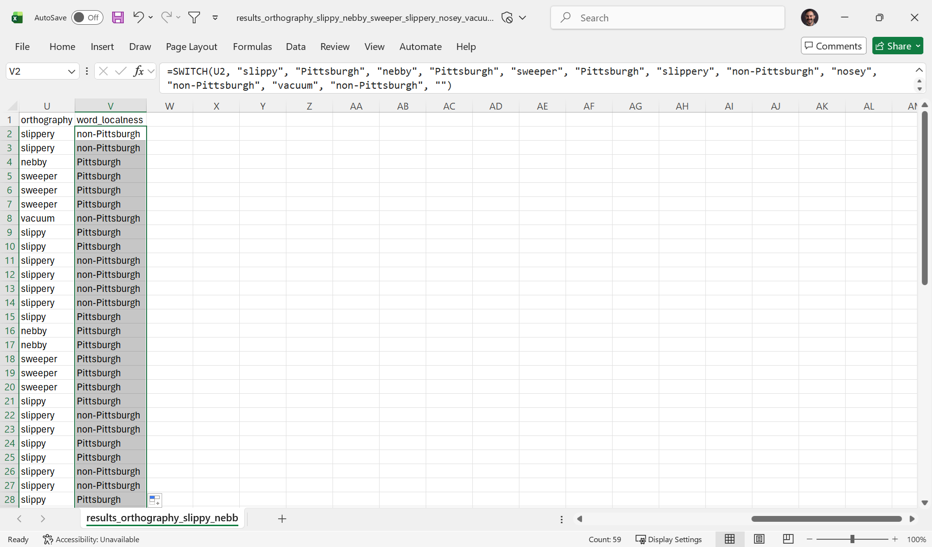
And here’s what it looks like if we press Enter/Return, then double-click the fill handle to apply the formula to the rest of the column:
Another example of categorizing is taking continuous measurements from a numeric layer and putting them into a smaller number of categories (also called “binning”). Sometimes, binning a continuous measure can be useful for analyzing and/or visualizing patterns in data. In this case, we’ll create a relative_speech_rate column by comparing the speech_rate of the utterance in which each token was found to the participant’s overall speech_rate across all their utterances. If the utterance speech_rate is greater (faster) than the participant’s overall speech_rate, we’ll say the relative_speech_rate is fast; otherwise, we’ll say it’s slow.
First, we’ll create a new relative_speech_rate column to the right of speech_rate. Then, we’ll create a formula using the IF function, which fills in one of two values based on a true-false statement (one value if the statement is true, the other if it’s false). Specifically, we’ll select cell R2 and type =IF(Q2 > P2, "fast", "slow"):
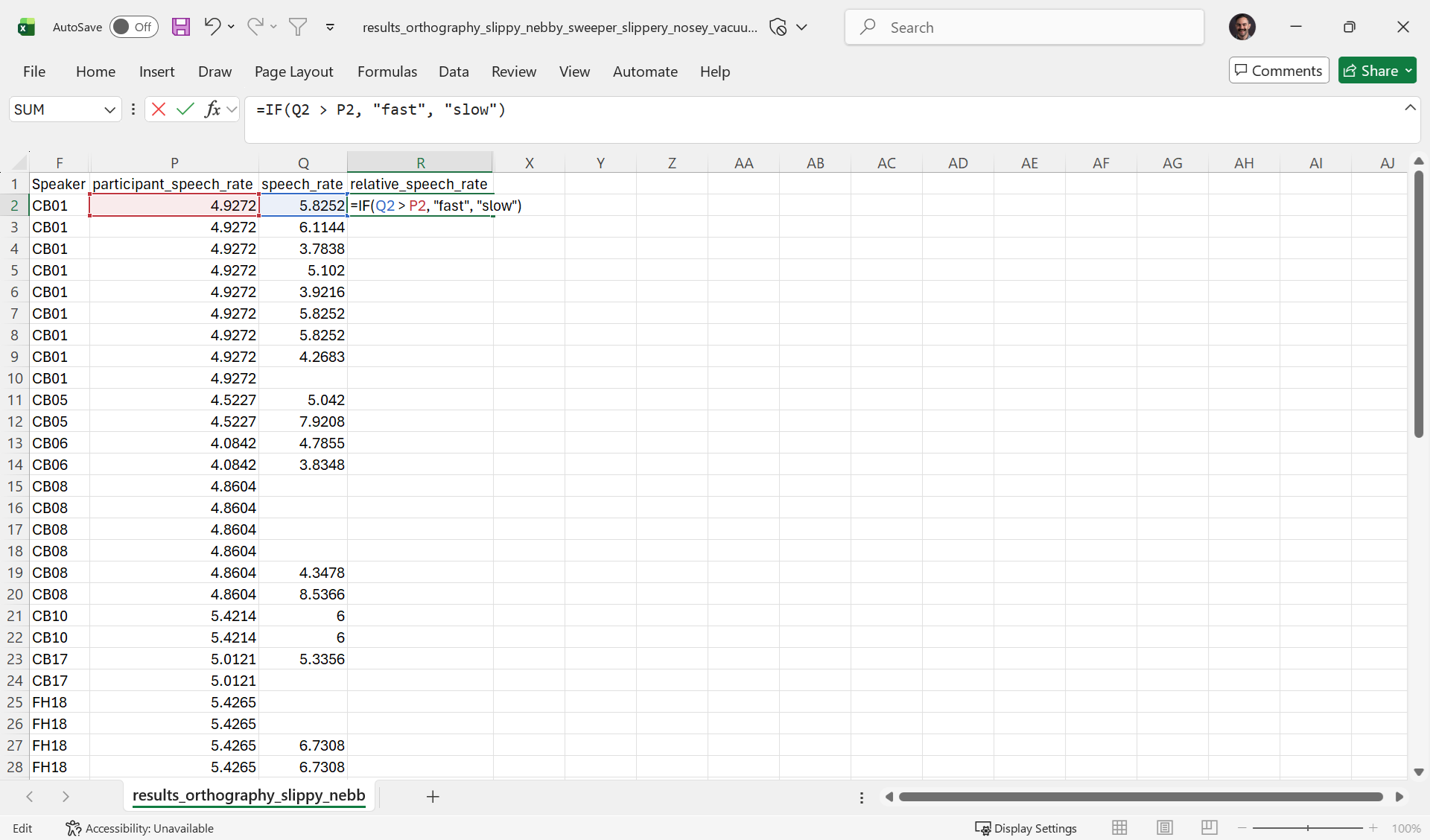
As you can see, Excel is using two different colors to highlight the two cells that the formula refers to: P2 and Q2.
Here’s what it looks like if we press Enter/Return, then double-click the fill handle to apply the formula to the rest of the column:
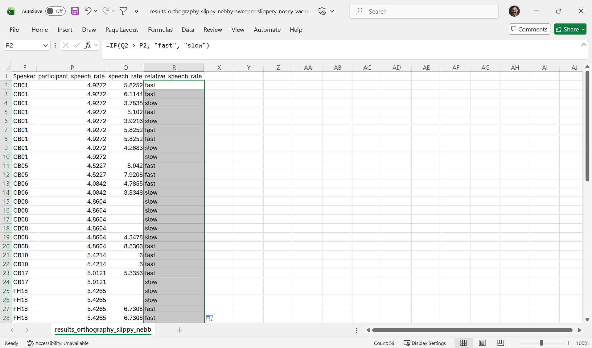
However, we’ve got a bit of a problem here. The token in row 10 is being marked as slow even though there’s no speech_rate in cell Q10. This is because the statement “this token’s speech_rate is greater than its participant_speech_rate” (Q10 > P10) is false—even though the reason it’s false is that this token doesn’t have a speech_rate. In other words, Excel doesn’t have the situational awareness to know that the comparison Q10 > P10 is meaningless because Q10 is blank.
As a segment-dependent layer, speech_rate has missing annotations for any utterance without segment annotations.
To deal with blanks, we need Excel to compare speech_rate to participant_speech_rate only if speech_rate is not blank. We do this by wrapping the original IF(...) statement (without the leading =) in another IF; within this “wrapper” IF, we use the ISBLANK function to check for a blank speech_rate. Putting it all together, the formula is =IF(ISBLANK(Q2), "", IF(Q2 > P2, "fast", "slow")):
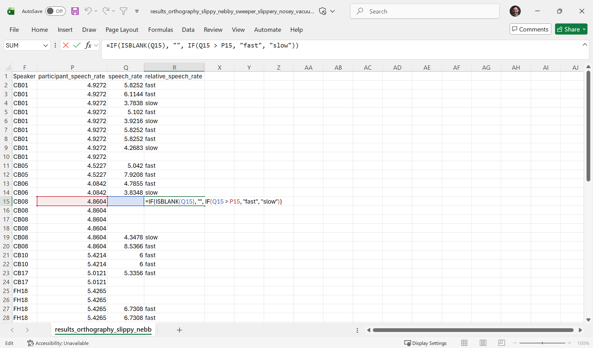
As you can see, in all the rows with blanks in the speech_rate column are also blank for relative_speech_rate.
Let’s say instead of putting
relative_speech_rateinto two bins, you wanted to just calculate a ratio of utterance speech_rate to participant speech_rate. In this case, you would just replace the innerIFwith an arithmetic expression:=IF(ISBLANK(Q2), "", Q2 / P2).